Using R to Analyze Zoom Recordings

UPDATE: 2021-05-13: zoomGroupStats is now available as a package on CRAN.


# To use the stable release version of zoomGroupStats, use:
install.packages("zoomGroupStats")

# To use the development version, which will be regularly updated with new functionality, use:
library(devtools)
install_github("https://github.com/andrewpknight/zoomGroupStats")

You can stay up-to-date on the latest functionality on http://zoomgroupstats.org.

UPDATE: 2021-04-30: In response to prodding from several folks who have been using the functions, I have started to build these R functions for analyzing Zoom meetings as a package. I’m grateful for all of the feedback and suggestions for features and modifications to this project. Although things are still in flux, you can now access a package version of zoomGroupStats. The easiest way is to use the dev_tools package and install the current development version from my github repository. To do so, you can run:


library(devtools)
install_github("https://github.com/andrewpknight/zoomGroupStats", force=TRUE)
library(zoomGroupStats)

I have created a multi-part guide for using this package to conduct research using Zoom and analyze data from Zoom, which I will continue to extend and elaborate. To keep up-to-date on this work, please use the dedicated package website http://zoomgroupstats.org.

Please keep the feedback and comments coming!

UPDATE: 2021-02-12: I’ve updated several items in the package. I’m also going to moving the development and updates all over to github to ease version control and documentation. For now, here is a post that is from a recent live tutorial session I facilitated. Stay tuned!

UPDATE: 2020-07-27: The new file contains some alpha-stage functions for doing audio transcription and for conducting a windowed conversation analysis. I haven’t yet tested these functions extensively or commented the windowed conversation analysis. Once COVID teaching planning eases, I’ll get back in an update further.

UPDATE: 2020-04-14: I added a new function (textConversationAnalysis) that gives some very basic and descriptive conversation metrics from either the video transcript or the chat file.

You can always access the most recent version of the functions by including the statement source(“http://apknight.org/zoomGroupStats.R”) at the top of your code.

Alternatively, you could go to http://apknight.org/zoomGroupStats.R and copy/paste the code into your editor.

ORIGINAL POST FOLLOWS:

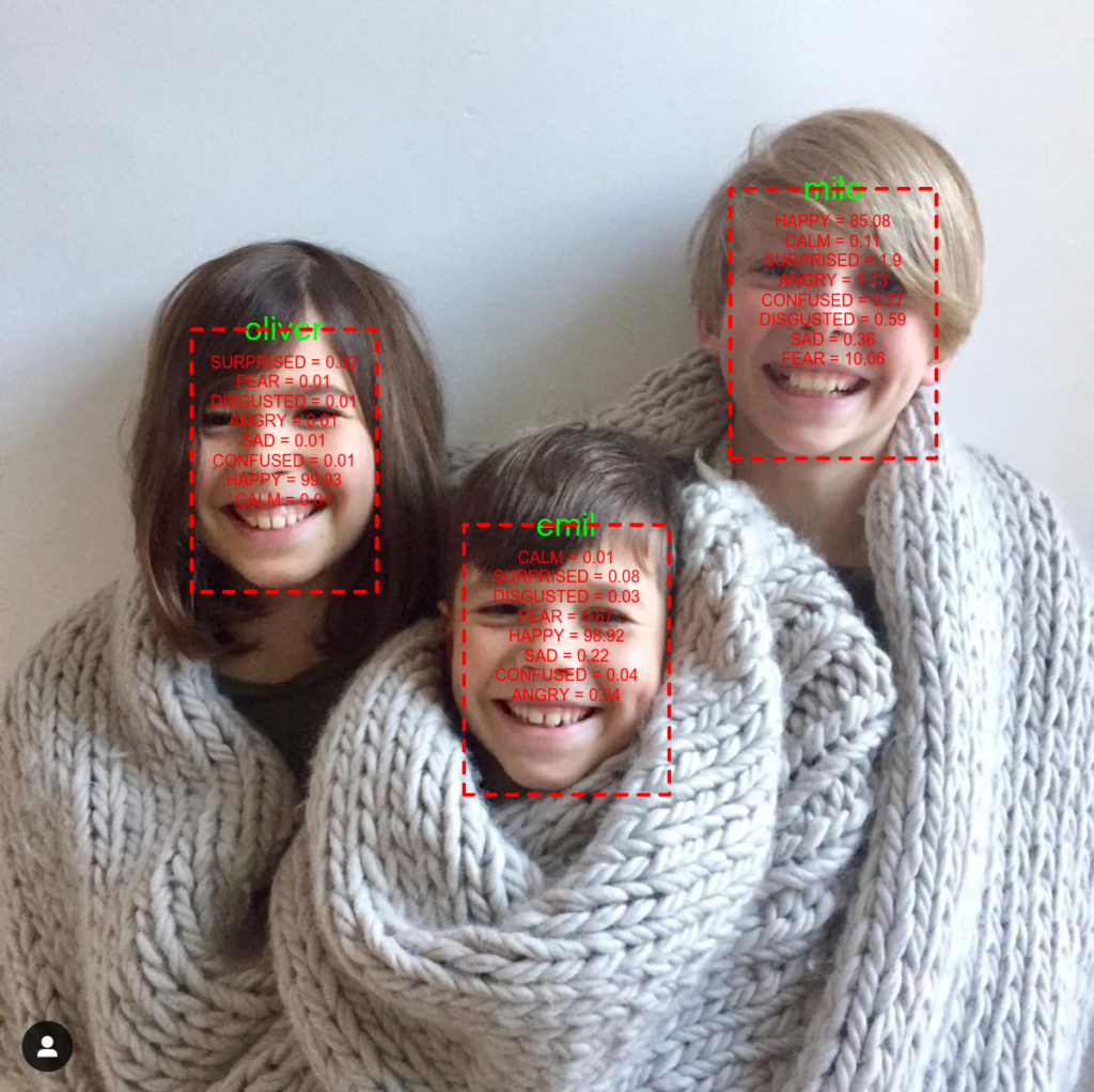
In response to the shift to so many online meetings, I created a set of R functions to help do research using web-based meetings. In brief, these functions use the output of recorded sessions (e.g., video feed, transcript file, chat file) to do things like sentiment analysis, face analysis, and emotional expression analysis. In the coming week, I will extend these to do basic conversation analysis (e.g., who speaks/chats most, turntaking).

I went overboard in commenting the code so that hopefully others can use them. But, if you’re still having trouble getting them to work, please don’t hesitate to reach out to me.

You can directly access the functions here:
http://apknight.org/zoomGroupStats.R

After reviewing this, you could call these functions using the following statement in R: source(“http://apknight.org/zoomGroupStats.R”)

Using R for Face Detection through AWS Rekognition

Today I experimented a little with the Rekognition service that AWS offers. I started out by experimenting with doing a Python version of this project, following this K-pop Idol Identifier with Rekognition post. It was pretty easy to setup; however, I tend to use R more than Python for data analysis and manipulation.

I found the excellent paws package, which is available through CRAN. The documentation for the paws package is very good, organized in an attractive github site here.

To start, I just duplicated the Python project in R, which was fairly straightforward. Then, I expanded on it a bit to annotate a photo with information about the emotional expressions being displayed by any subjects. The annotated image above shows what the script outputs if it is given a photo of my kids. And, here’s the commented code that walks through what I did.

########################
# Setup the environment with libraries and the key service
########################

# Use the paws library for easy access to aws
# Note: You will need to authenticate. For this project, I have my credentials in an
# AWS configuration; so, paws looks there for them.
# paws provides good information on how to do this:
# https://github.com/paws-r/paws/blob/master/docs/credentials.md
library(paws)

# Use the magick library for image functions.
library(magick)

# This application is going to use the rekognition service from AWS. The paws documentation is here:
# # https://paws-r.github.io/docs/rekognition/
svc <- rekognition()

########################
# First, create a new collection that you will use to store the set of identified faces. This will be
# the library of faces that you use for determining someone's identity
########################

# I am going to create a collection for a set of family photos
svc$create_collection(CollectionId = "family-r")

# I stored a set of faces of my kids in a single directory on my Desktop. Inside
# this directory are multiple photos of each person, with the filename set as personname_##.png. This
# means that there are several photos per kid, which should help with classification.

# Get the list of files
path = "~/Desktop/family"
file.names = dir(path, full.names=F)

# Loop through the files in the specified folder, add and index them in the collection
for(f in file.names) {
    imgFile = paste(path,f,sep="/")
    # This gets the name of the kid, which is embedded in the filename and separated from the number with an underscore
    imgName = unlist(strsplit(f,split="_"))[[1]]
    # Add the photos and the name to the collection that I created
    svc$index_faces(CollectionId="family-r", Image=list(Bytes=imgFile), ExternalImageId=imgName, DetectionAttributes=list())
}

########################
# Second, take a single photo that has multiple kids in it. Label each kid with his name and the
# emotions that are expressed in the photo.
########################

# Get information about a group photo
grp.photo = "~/Desktop/all_three_small.png"

# Read the photo using magick
img = image_read(grp.photo)

# Get basic informatino about the photo that will be useful for annotating
inf = image_info(img)

# Detect the faces in the image and pull all attributes associated with faces
o = svc$detect_faces(Image=list(Bytes=grp.photo), Attributes="ALL")

# Just get the face details
all_faces = o$FaceDetails
length(all_faces)

# Loop through the faces, one by one. For each face, draw a rectangle around it, add the kid's name, and emotions

# Duplicate the original image to have something to annotate and output
new.img = img

for(face in all_faces) {

    # Prepare a label that collapses across the emotions data provided by rekognition. Give the type of
    # emotion and the confidence that AWS has in its expression.
    emo.label = ""
    for(emo in face$Emotions) {
        emo.label = paste(emo.label,emo$Type, " = ", round(emo$Confidence, 2), "\n", sep="")
    }

    # Identify the coordinates of the face. Note that AWS returns percentage values of the total image size. This is
    # why the image info object above is needed
    box = face$BoundingBox
    image_width=inf$width
    image_height=inf$height
    x1 = box$Left*image_width
    y1 = box$Top*image_height
    x2 = x1 + box$Width*image_width
    y2 = y1 + box$Height*image_height  

    # Create a subset image in memory that is just cropped around the focal face
    img.crop = image_crop(img, paste(box$Width*image_width,"x",box$Height*image_height,"+",x1,"+",y1, sep=""))
    img.crop = image_write(img.crop, path = NULL, format = "png")

    # Search in a specified collection to see if we can label the identity of the face is in this crop
    o = svc$search_faces_by_image(CollectionId="family-r",Image=list(Bytes=img.crop), FaceMatchThreshold=70)

    # Create a graphics device version of the larger photo that we can annotate
    new.img = image_draw(new.img)

    # If the face matches something in the collection, then add the name to the image
    if(length(o$FaceMatches) > 0) {
        faceName = o$FaceMatches[[1]]$Face$ExternalImageId
        faceConfidence = round(o$FaceMatches[[1]]$Face$Confidence,3)
        print(paste("Detected: ",faceName, sep=""))
        # Annotate with the name of the person
        text(x=x1+(box$Width*image_width)/2, y=y1,faceName, adj=0.5, cex=3, col="green")
    }

    # Draw a rectangle around the face
    rect(x1,y1,x2,y2, border="red", lty="dashed", lwd=5)   

    # Annotate the photo with the emotions information
    text(x=x1+(box$Width*image_width)/2, y=y1+50,emo.label, pos=1, cex=1.5, col="red")     

    dev.off()
}

# Write the image out to file
image_write(new.img, path="~/Desktop/annotated_image.png", format="png")

Using R to Analyze Twitter

The code below will give you a start on processing text data from Twitter. There are some basic examples of how to pull down tweets for selected users and compare/contrast the sentiment of their posts.

#####################
# This script illustrates how to pull data from
# twitter and use default settings for English
# language sentiment analysis
#####################
library(twitteR)
library(rtweet)
library(syuzhet)
library(ngram)
library(reshape2)
require(dplyr)
library(timeDate)
library(ggplot2)

#####################
# This is just a crude string cleaning function for the purposes
# of illustration.
#####################

clean.string <- function(string){
    # Lowercase
    temp <- tolower(string)
    # Remove everything that is not a number or letter (may want to keep more
    # stuff in your actual analyses).
    temp <- stringr::str_replace_all(temp,"[^a-zA-Z\\s]", " ")
    # Shrink down to just one white space
    temp <- stringr::str_replace_all(temp,"[\\s]+", " ")
    return(temp)
}

#####################
# this function returns a crude sentiment analysis of the tweets from a set of
# users' timelines. You must provide a vector of users.
#####################

twit.sentiment <- function(users, n.tweets=200, include.retweet=FALSE) {
    sent.vars = c("anger", "anticipation", "disgust", "fear", "joy", "sadness", "surprise", "trust", "negative", "positive")   
    d.vars = c("user_id", "screen_name", "created_at", "retweet_count", "favorite_count", "followers_count", "friends_count", "text")
    d = data.frame(get_timelines(users, n=n.tweets, parse=TRUE))

    # do a very light text cleaning
    d$text_clean = unlist(lapply(d$text, clean.string))

    # count the clean words
    d$n_words = unlist(lapply(d$text_clean, wordcount))

    # Do the sentiment analysis using nrc. In a real production sentiment analysis, you would want
    # to consider several different dictionaries. Check out the following page for a walkthrough of
    # some of the different lexicons you might consider:
    # https://cran.r-project.org/web/packages/syuzhet/vignettes/syuzhet-vignette.html
    d[,sent.vars] = bind_rows(lapply(d$text_clean, get_nrc_sentiment))
    head(d)

    # Get a percentage of pos/neg by number of words in the email
    d$neg_pct = d$negative/d$n_words
    d$pos_pct = d$positive/d$n_words

    if(include.retweet) {
        d.sub = d[,c(d.vars, sent.vars)]       
    } else {
        d.sub = d[!(d$is_retweet),c(d.vars, sent.vars)]    
    }
    return(d.sub)
}

#####################
# Explore the dictionaries, showing how different
# words are coded
#####################

nrc = get_sentiment_dictionary(dictionary = "nrc", language = "english")
syuzhet = get_sentiment_dictionary(dictionary = "syuzhet", language = "english")

nrc[nrc$word == "horrible", ]
syuzhet[syuzhet$word == "horrible", ]

nrc[nrc$word == "disastrous", ]
syuzhet[syuzhet$word == "disastrous", ]

#####################
# Exploring sentiment analysis
#####################

v1 = "Man, I am having the best day today. The sun is out and it is a beautiful day."
v2 = "So grateful to be part of this supportive community. This is an amazing place to work."
v3 = "What a horrible day. Not only is it storming, but I fell in the mud and broke my phone."
v4 = "Awful bosses and terrible co-workers. This is a ridiculously bad place to work."

v5 = "I am not having the best day today. The sun is not out and it is not a beautiful day."
v6 = "Some days are better than others. This is the latter."
v7 = "So, got my final back. Um, yeah. The professor sure knows how to give the gift of a great day."
v8 = "Great idea Olin...Make all the students swipe their cards just to get onto the 4th floor. Beautiful building that we can't access."

get_nrc_sentiment(clean.string(v1))
get_nrc_sentiment(clean.string(v2))
get_nrc_sentiment(clean.string(v3))
get_nrc_sentiment(clean.string(v4))
get_nrc_sentiment(clean.string(v5))
get_nrc_sentiment(clean.string(v6))
get_nrc_sentiment(clean.string(v7))
get_nrc_sentiment(clean.string(v8))

#####################
# The first thing you need to do is create an app for your twitter account
# you can find instructions here:
# https://developer.twitter.com/en/docs/basics/apps/overview.html

# Once you've created an app, then add the following information to this script
#####################
# twitter_consumer_key = "YOUR INFO HERE"
# twitter_consumer_secret = "YOUR INFO HERE"
# twitter_access_token = "YOUR INFO HERE"
# twitter_access_secret = "YOUR INFO HERE"

setup_twitter_oauth(twitter_consumer_key, twitter_consumer_secret, twitter_access_token, twitter_access_secret)

#####################
# Sample sentiment analysis on accounts where
# we have strong priors about their sentiment
#####################

sad_happy = c("sosadtoday", "angrymemorys", "gohappiest", "kindnessgirl")
d.sh = twit.sentiment(users=sad_happy, n.tweets=200, include.retweet=F)
boxplot(positive~screen_name, data=d.sh, cex.axis=.7, las=2, main="positive")
boxplot(negative~screen_name, data=d.sh, cex.axis=.7, las=2, main="negative")

#####################
# Illustrating the potential for looking at specific users and
# comparing / contrasting individual employees' sentiment
#####################

OlinPeeps = c("DeanTaylorWashU", "sjmalter", "LamarPierce1", "OrgStratProf")
BSchoolDeans = c("DeanTaylorWashU", "scottderue")
BSchools = c("OlinBusiness", "Wharton")

d.olin = twit.sentiment(users=OlinPeeps, n.tweets=300, include.retweet=F)
d.deans = twit.sentiment(users=BSchoolDeans, n.tweets=300, include.retweet=F)
d.schools = twit.sentiment(users=BSchools, n.tweets=300, include.retweet=F)

boxplot(positive~screen_name, data=d.olin, cex.axis=.7, las=2, main="positive")
boxplot(negative~screen_name, data=d.olin, cex.axis=.7, las=2, main="negative")

boxplot(positive~screen_name, data=d.deans, cex.axis=.7, las=2, main="positive")
boxplot(negative~screen_name, data=d.deans, cex.axis=.7, las=2, main="negative")

boxplot(positive~screen_name, data=d.schools, cex.axis=.7, las=2, main="positive")
boxplot(negative~screen_name, data=d.schools, cex.axis=.7, las=2, main="negative")

#####################
# Illustrating the potential for looking at trends over time
#####################
olin.all = c("DeanTaylorWashU", "sjmalter", "LamarPierce1", "OrgStratProf", "sethcarnahan", "peterboumgarden",
    "jrobmartin", "milbourn_todd", "danbentle", "wustlbusiness", "drpatsportsbiz", "analisaortiz", "krwools")

d.lrg = twit.sentiment(users=olin.all, n.tweets=300, include.retweet=F)

d.lrg$date = as.Date(d.lrg$created_at)
d.lrg$year = as.numeric(strftime(d.lrg$date, format="%Y"))
d.lrg$month = as.numeric(strftime(d.lrg$date, format="%m"))
d.lrg$woy = as.numeric(strftime(d.lrg$date, format="%V"))

o = aggregate(d.lrg[,c("positive", "negative")], by=list(d.lrg$year, d.lrg$month), mean)
names(o)[1:2] = c("year", "month")

plot(o[o$year == 2018, "month"], o[o$year == 2018, "positive"], type="l", ylim=c(0,3), col="dark green", lwd=3, ylab="sentiment", xlab="month")
lines(o[o$year == 2017, "month"], o[o$year == 2017, "positive"], type="l", col="dark green", lwd=3, lty=2)

lines(o[o$year == 2018, "month"], o[o$year == 2018, "negative"], type="l", col="dark red", lwd=3)
lines(o[o$year == 2017, "month"], o[o$year == 2017, "negative"], type="l", col="dark red", lwd=3, lty=2)

boxplot(positive~screen_name, data=d.lrg, cex.axis=.7, las=2, main="positive")
boxplot(negative~screen_name, data=d.lrg, cex.axis=.7, las=2, main="negative")

d.lrg$name = as.factor(d.lrg$screen_name)

p <- ggplot(d.lrg, aes(x=name, y=positive)) + geom_violin()
p <- ggplot(d.lrg, aes(x=name, y=negative)) + geom_violin()

d.lrg[d.lrg$negative > 7, ]

Sentiment analysis on Gmail with R: The gmailr package

For today’s exploration, I wanted to connect to my gmail account, pull messages, and do a quick sentiment analysis on the text. The focus of this code is pulling and transforming the data from gmail’s api–not doing a precise and polished sentiment analysis. I wanted to learn a bit about the gmail api the gmailr package (which right now is pretty thin on documentation).

There is much potential with this. The api would make everything from sentiment analysis to network analysis on your own gmail account possible.

##########################################
# This script gives an example of how to connect
# to a personal gmail account, extract a set of messages
# and do a quick-and-dirty sentiment analysis on the
# body of the messages.
# NOTE: This is not a pure or clean analysis of this text data.
# For production, you would want to make sure to clean up the
# body of the text data (e.g., ensuring that you don't have duplicate
# messages that are appended at the bottom of replies).
#
# However, this should give you a place to start for making sense of your email.
##########################################


#### -- ## -- ## -- ## -- ## -- ## -- ## -- ## -- ####
## Setup
#### -- ## -- ## -- ## -- ## -- ## -- ## -- ## -- ####
# Setup your environment, marking a particular working directory where you'd like
# to output files and loading libraries that you'll use
# syuzhet has a set of functions for doing sentiment analysis
library(syuzhet)
# ngram is useful for breaking up and parsing text data
library(ngram)
# reshape2 is also helpul for parsing text data
library(reshape2)
# use this to smash a list
require(dplyr)
# gmailr has a set of functions for connecting to gmail and parsing emails
library(gmailr)


## User-defined function for doing a quick-and-dirty clean-up on text
# You could add elements to this to create an even more precise set of
# text data to parse for your sentiment analysis. For a production
# text analysis, you would want to create a clean set of data.

clean.string <- function(string){
    # Lowercase
    temp <- tolower(string)
    # Remove everything that is not a number or letter (may want to keep more
    # stuff in your actual analyses).
    temp <- stringr::str_replace_all(temp,"[^a-zA-Z\\s]", " ")
    # Shrink down to just one white space
    temp <- stringr::str_replace_all(temp,"[\\s]+", " ")
    return(temp)
}

## User-defined function for pulling a set of messages from gmail
# and doing a sentiment analysis on those messages. This will also retain the actual
# body of the messages in case you want to do something further with it down
# the line. The only input into the function is a vector of message ids
# that you want to pull and process.


gmail.sentiment = function(ids) {

    # a vector of the sentiment variables
    sent.vars = c("anger", "anticipation", "disgust", "fear", "joy", "sadness", "surprise", "trust", "negative", "positive")
    # a vector of the email vars
    email.vars = c("id", "to", "from", "cc", "bcc", "date", "subject", "body") 
    # put together and also add the number of words in the body
    all.vars = c(email.vars, "n_words", sent.vars)

    null.to.na = function(x) {
        x = ifelse(is.null(x), NA, x)
        return(x)
    }

    # Loop through the vector of message ids and pull the info for that specific message
    # We're creating a data.frame here that contains the information for this query of messages
    for(i in 1:length(ids)) {

        # Get the header info for the message, replacing any null values with NA
        id = ids[i]
        msg = message(id)
        to = to(msg)
        to = null.to.na(to)
        from = from(msg)
        from = null.to.na(from)    
        cc = cc(msg)
        cc = null.to.na(cc)
        bcc = bcc(msg)
        bcc = null.to.na(bcc)      
        date = date(msg)
        date = null.to.na(date)
        subject = subject(msg)
        subject = null.to.na(subject)  
        body = unlist(body(msg))
        body = null.to.na(body)

        # Create a holding line
        res.line = data.frame(cbind(id, to, from, cc, bcc, date, subject, body), stringsAsFactors=F)

        # if this is the first pass through, then create an outset. Otherwise, append this line
        # to the existing outset
        if(i == 1) {
            res.out = res.line
        } else {
            res.out = rbind(res.out, res.line)
        }
    }

    # do a very light text cleaning
    res.out$body_clean = unlist(lapply(res.out$body, clean.string))

    # count the clean words
    res.out$n_words = unlist(lapply(res.out$body_clean, wordcount))
   
    # Do the sentiment analysis using nrc. In a real production sentiment analysis, you would want
    # to consider several different dictionaries. Check out the following page for a walkthrough of
    # some of the different lexicons you might consider:
    # https://cran.r-project.org/web/packages/syuzhet/vignettes/syuzhet-vignette.html
    res.out[,sent.vars] = bind_rows(lapply(res.out$body_clean, get_nrc_sentiment))

    # Get a percentage of pos/neg by number of words in the email
    res.out$neg_pct = res.out$negative/res.out$n_words
    res.out$pos_pct = res.out$positive/res.out$n_words

    # parse the date information into some variables to use in graphing
    res.out$dow = substr(res.out$date, 1, 3)   

    res.out$date_time = substr(res.out$date, 6, nchar(res.out$date))
    o = colsplit(trimws(res.out$date_time), " ", names=c("day", "month", "year", "time", "offset"))
    d = cbind(res.out, o)
    d$date_time_format = as.Date(paste(d$month, " ", as.numeric(d$day), " ", as.numeric(d$year), sep=""), format="%b %d %Y")
    d$month_num = as.numeric(substr(d$date_time_format, 6,7))
    d$day_num = as.numeric(substr(d$date_time_format, 9,10))

    return(d)
}

#### -- ## -- ## -- ## -- ## -- ## -- ## -- ## -- ####
## Connect to gmail
#### -- ## -- ## -- ## -- ## -- ## -- ## -- ## -- ####

## Note, you will need to create your own application to connect to gmail
## Here are some steps for doing this:
## 1. Go to https://console.developers.google.com/
## 2. Create a new project
## 3. Copy-and-paste the Client ID and Client Secret into the fields below
## 4. Add an authorized redirect URI: http://localhost:1410/

client_id = "{INSERT YOUR ID HERE}"
client_secret = "{INSERT YOUR SECRET HERE}"

# Running this will open a web browser and ask you to authenticate
# If you are already authenticated into gmail, it will just give you a confirmation
# message, indicating that you are authenticated. You can close the browser and begin using gmail
# NOTE: After a period of time, your authentication will time-out. When you try to pass
# a request to gmail, you'll get an error. Just re-run the line below and you'll re-authenticate.
gmail_auth(scope="read_only", id=client_id, secret=client_secret)

#### -- ## -- ## -- ## -- ## -- ## -- ## -- ## -- ####
## Request a set of message ids that match a given query.
## There are many slick ways to search for messages (or threads) in gmail. Any of these methods can be used
## in the search=" " argument.
## For a full set of search options, check out this page:
## https://support.google.com/mail/answer/7190?hl=en
#### -- ## -- ## -- ## -- ## -- ## -- ## -- ## -- ####

## For this example, I'm going to pull all messages that I sent (i.e., those that gmail auto-labeled as SENT)
## I'm going to specify a particular time window and a maximum of 10k messages.
msgs = messages(search="before:2019/01/01 after:2005/12/01", num_results = 10000, label_ids="SENT")

# the messages function abovewill return an object with thread and message ids. The function below
# will return a vector of string ids that can be used in subsequent pulls.
# Note that because the function has to call each message, this can take sometime to process
# So, if you have something like 4000 messages, expect for it to take several minutes to finish running.
# Be patient! It's not efficient code.
ids = gmailr::id(msgs, what="message_id")
o = gmail.sentiment(ids)

# Because this took so long to do, I'm going to write out the results
write.table(o, "./gmail_text_analysis.csv", sep=",", row.names=F)

#### -- ## -- ## -- ## -- ## -- ## -- ## -- ## -- ####
# At this point, you can use your favorite graphing and analysis tools
# to analyze this dataset at different levels of analysis (e.g., time, day, day of week, month, year)
#### -- ## -- ## -- ## -- ## -- ## -- ## -- ## -- ####