Using R for Face Detection through AWS Rekognition

Today I experimented a little with the Rekognition service that AWS offers. I started out by experimenting with doing a Python version of this project, following this K-pop Idol Identifier with Rekognition post. It was pretty easy to setup; however, I tend to use R more than Python for data analysis and manipulation.

I found the excellent paws package, which is available through CRAN. The documentation for the paws package is very good, organized in an attractive github site here.

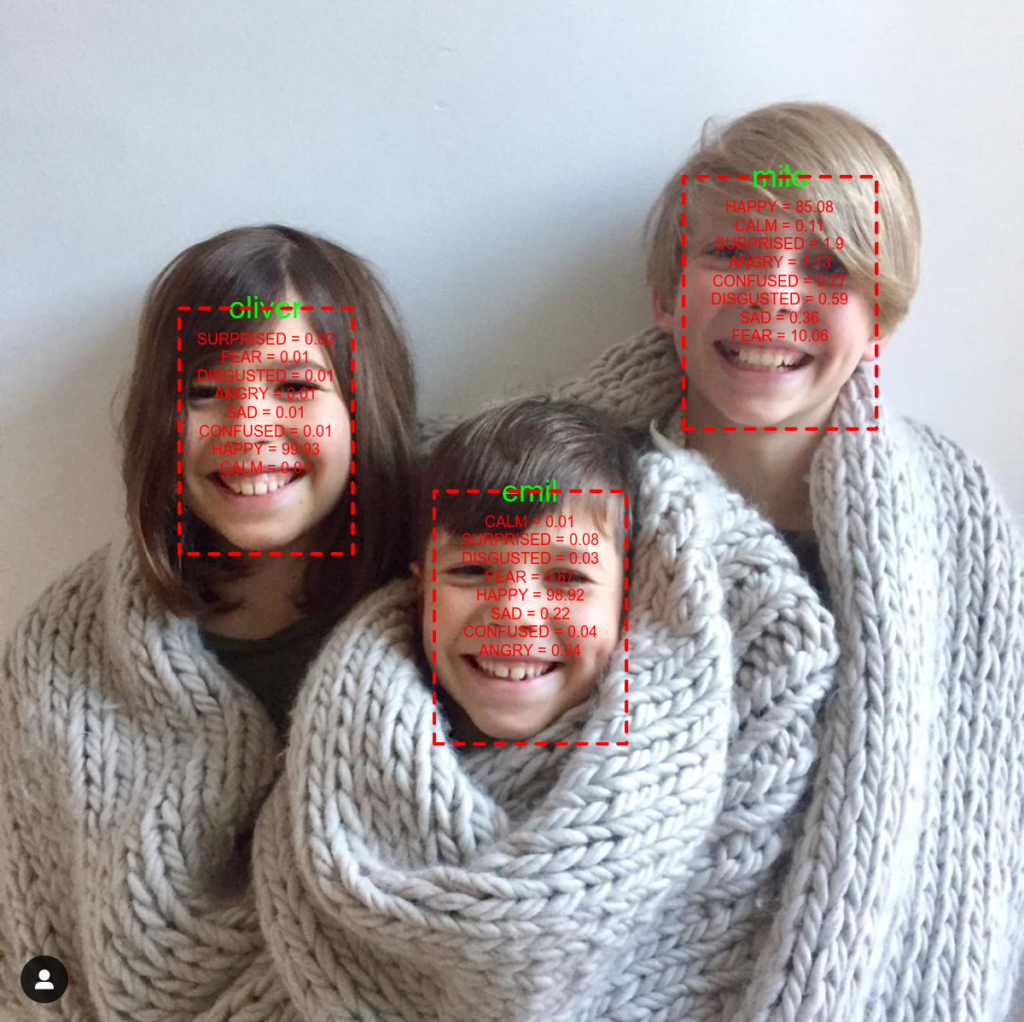
To start, I just duplicated the Python project in R, which was fairly straightforward. Then, I expanded on it a bit to annotate a photo with information about the emotional expressions being displayed by any subjects. The annotated image above shows what the script outputs if it is given a photo of my kids. And, here’s the commented code that walks through what I did.

########################
# Setup the environment with libraries and the key service
########################

# Use the paws library for easy access to aws
# Note: You will need to authenticate. For this project, I have my credentials in an
# AWS configuration; so, paws looks there for them.
# paws provides good information on how to do this:
# https://github.com/paws-r/paws/blob/master/docs/credentials.md
library(paws)

# Use the magick library for image functions.
library(magick)

# This application is going to use the rekognition service from AWS. The paws documentation is here:
# # https://paws-r.github.io/docs/rekognition/
svc <- rekognition()

########################
# First, create a new collection that you will use to store the set of identified faces. This will be
# the library of faces that you use for determining someone's identity
########################

# I am going to create a collection for a set of family photos
svc$create_collection(CollectionId = "family-r")

# I stored a set of faces of my kids in a single directory on my Desktop. Inside
# this directory are multiple photos of each person, with the filename set as personname_##.png. This
# means that there are several photos per kid, which should help with classification.

# Get the list of files
path = "~/Desktop/family"
file.names = dir(path, full.names=F)

# Loop through the files in the specified folder, add and index them in the collection
for(f in file.names) {
    imgFile = paste(path,f,sep="/")
    # This gets the name of the kid, which is embedded in the filename and separated from the number with an underscore
    imgName = unlist(strsplit(f,split="_"))[[1]]
    # Add the photos and the name to the collection that I created
    svc$index_faces(CollectionId="family-r", Image=list(Bytes=imgFile), ExternalImageId=imgName, DetectionAttributes=list())
}

########################
# Second, take a single photo that has multiple kids in it. Label each kid with his name and the
# emotions that are expressed in the photo.
########################

# Get information about a group photo
grp.photo = "~/Desktop/all_three_small.png"

# Read the photo using magick
img = image_read(grp.photo)

# Get basic informatino about the photo that will be useful for annotating
inf = image_info(img)

# Detect the faces in the image and pull all attributes associated with faces
o = svc$detect_faces(Image=list(Bytes=grp.photo), Attributes="ALL")

# Just get the face details
all_faces = o$FaceDetails
length(all_faces)

# Loop through the faces, one by one. For each face, draw a rectangle around it, add the kid's name, and emotions

# Duplicate the original image to have something to annotate and output
new.img = img

for(face in all_faces) {

    # Prepare a label that collapses across the emotions data provided by rekognition. Give the type of
    # emotion and the confidence that AWS has in its expression.
    emo.label = ""
    for(emo in face$Emotions) {
        emo.label = paste(emo.label,emo$Type, " = ", round(emo$Confidence, 2), "\n", sep="")
    }

    # Identify the coordinates of the face. Note that AWS returns percentage values of the total image size. This is
    # why the image info object above is needed
    box = face$BoundingBox
    image_width=inf$width
    image_height=inf$height
    x1 = box$Left*image_width
    y1 = box$Top*image_height
    x2 = x1 + box$Width*image_width
    y2 = y1 + box$Height*image_height  

    # Create a subset image in memory that is just cropped around the focal face
    img.crop = image_crop(img, paste(box$Width*image_width,"x",box$Height*image_height,"+",x1,"+",y1, sep=""))
    img.crop = image_write(img.crop, path = NULL, format = "png")

    # Search in a specified collection to see if we can label the identity of the face is in this crop
    o = svc$search_faces_by_image(CollectionId="family-r",Image=list(Bytes=img.crop), FaceMatchThreshold=70)

    # Create a graphics device version of the larger photo that we can annotate
    new.img = image_draw(new.img)

    # If the face matches something in the collection, then add the name to the image
    if(length(o$FaceMatches) > 0) {
        faceName = o$FaceMatches[[1]]$Face$ExternalImageId
        faceConfidence = round(o$FaceMatches[[1]]$Face$Confidence,3)
        print(paste("Detected: ",faceName, sep=""))
        # Annotate with the name of the person
        text(x=x1+(box$Width*image_width)/2, y=y1,faceName, adj=0.5, cex=3, col="green")
    }

    # Draw a rectangle around the face
    rect(x1,y1,x2,y2, border="red", lty="dashed", lwd=5)   

    # Annotate the photo with the emotions information
    text(x=x1+(box$Width*image_width)/2, y=y1+50,emo.label, pos=1, cex=1.5, col="red")     

    dev.off()
}

# Write the image out to file
image_write(new.img, path="~/Desktop/annotated_image.png", format="png")

Using R to Analyze Twitter

The code below will give you a start on processing text data from Twitter. There are some basic examples of how to pull down tweets for selected users and compare/contrast the sentiment of their posts.

#####################
# This script illustrates how to pull data from
# twitter and use default settings for English
# language sentiment analysis
#####################
library(twitteR)
library(rtweet)
library(syuzhet)
library(ngram)
library(reshape2)
require(dplyr)
library(timeDate)
library(ggplot2)

#####################
# This is just a crude string cleaning function for the purposes
# of illustration.
#####################

clean.string <- function(string){
    # Lowercase
    temp <- tolower(string)
    # Remove everything that is not a number or letter (may want to keep more
    # stuff in your actual analyses).
    temp <- stringr::str_replace_all(temp,"[^a-zA-Z\\s]", " ")
    # Shrink down to just one white space
    temp <- stringr::str_replace_all(temp,"[\\s]+", " ")
    return(temp)
}

#####################
# this function returns a crude sentiment analysis of the tweets from a set of
# users' timelines. You must provide a vector of users.
#####################

twit.sentiment <- function(users, n.tweets=200, include.retweet=FALSE) {
    sent.vars = c("anger", "anticipation", "disgust", "fear", "joy", "sadness", "surprise", "trust", "negative", "positive")   
    d.vars = c("user_id", "screen_name", "created_at", "retweet_count", "favorite_count", "followers_count", "friends_count", "text")
    d = data.frame(get_timelines(users, n=n.tweets, parse=TRUE))

    # do a very light text cleaning
    d$text_clean = unlist(lapply(d$text, clean.string))

    # count the clean words
    d$n_words = unlist(lapply(d$text_clean, wordcount))

    # Do the sentiment analysis using nrc. In a real production sentiment analysis, you would want
    # to consider several different dictionaries. Check out the following page for a walkthrough of
    # some of the different lexicons you might consider:
    # https://cran.r-project.org/web/packages/syuzhet/vignettes/syuzhet-vignette.html
    d[,sent.vars] = bind_rows(lapply(d$text_clean, get_nrc_sentiment))
    head(d)

    # Get a percentage of pos/neg by number of words in the email
    d$neg_pct = d$negative/d$n_words
    d$pos_pct = d$positive/d$n_words

    if(include.retweet) {
        d.sub = d[,c(d.vars, sent.vars)]       
    } else {
        d.sub = d[!(d$is_retweet),c(d.vars, sent.vars)]    
    }
    return(d.sub)
}

#####################
# Explore the dictionaries, showing how different
# words are coded
#####################

nrc = get_sentiment_dictionary(dictionary = "nrc", language = "english")
syuzhet = get_sentiment_dictionary(dictionary = "syuzhet", language = "english")

nrc[nrc$word == "horrible", ]
syuzhet[syuzhet$word == "horrible", ]

nrc[nrc$word == "disastrous", ]
syuzhet[syuzhet$word == "disastrous", ]

#####################
# Exploring sentiment analysis
#####################

v1 = "Man, I am having the best day today. The sun is out and it is a beautiful day."
v2 = "So grateful to be part of this supportive community. This is an amazing place to work."
v3 = "What a horrible day. Not only is it storming, but I fell in the mud and broke my phone."
v4 = "Awful bosses and terrible co-workers. This is a ridiculously bad place to work."

v5 = "I am not having the best day today. The sun is not out and it is not a beautiful day."
v6 = "Some days are better than others. This is the latter."
v7 = "So, got my final back. Um, yeah. The professor sure knows how to give the gift of a great day."
v8 = "Great idea Olin...Make all the students swipe their cards just to get onto the 4th floor. Beautiful building that we can't access."

get_nrc_sentiment(clean.string(v1))
get_nrc_sentiment(clean.string(v2))
get_nrc_sentiment(clean.string(v3))
get_nrc_sentiment(clean.string(v4))
get_nrc_sentiment(clean.string(v5))
get_nrc_sentiment(clean.string(v6))
get_nrc_sentiment(clean.string(v7))
get_nrc_sentiment(clean.string(v8))

#####################
# The first thing you need to do is create an app for your twitter account
# you can find instructions here:
# https://developer.twitter.com/en/docs/basics/apps/overview.html

# Once you've created an app, then add the following information to this script
#####################
# twitter_consumer_key = "YOUR INFO HERE"
# twitter_consumer_secret = "YOUR INFO HERE"
# twitter_access_token = "YOUR INFO HERE"
# twitter_access_secret = "YOUR INFO HERE"

setup_twitter_oauth(twitter_consumer_key, twitter_consumer_secret, twitter_access_token, twitter_access_secret)

#####################
# Sample sentiment analysis on accounts where
# we have strong priors about their sentiment
#####################

sad_happy = c("sosadtoday", "angrymemorys", "gohappiest", "kindnessgirl")
d.sh = twit.sentiment(users=sad_happy, n.tweets=200, include.retweet=F)
boxplot(positive~screen_name, data=d.sh, cex.axis=.7, las=2, main="positive")
boxplot(negative~screen_name, data=d.sh, cex.axis=.7, las=2, main="negative")

#####################
# Illustrating the potential for looking at specific users and
# comparing / contrasting individual employees' sentiment
#####################

OlinPeeps = c("DeanTaylorWashU", "sjmalter", "LamarPierce1", "OrgStratProf")
BSchoolDeans = c("DeanTaylorWashU", "scottderue")
BSchools = c("OlinBusiness", "Wharton")

d.olin = twit.sentiment(users=OlinPeeps, n.tweets=300, include.retweet=F)
d.deans = twit.sentiment(users=BSchoolDeans, n.tweets=300, include.retweet=F)
d.schools = twit.sentiment(users=BSchools, n.tweets=300, include.retweet=F)

boxplot(positive~screen_name, data=d.olin, cex.axis=.7, las=2, main="positive")
boxplot(negative~screen_name, data=d.olin, cex.axis=.7, las=2, main="negative")

boxplot(positive~screen_name, data=d.deans, cex.axis=.7, las=2, main="positive")
boxplot(negative~screen_name, data=d.deans, cex.axis=.7, las=2, main="negative")

boxplot(positive~screen_name, data=d.schools, cex.axis=.7, las=2, main="positive")
boxplot(negative~screen_name, data=d.schools, cex.axis=.7, las=2, main="negative")

#####################
# Illustrating the potential for looking at trends over time
#####################
olin.all = c("DeanTaylorWashU", "sjmalter", "LamarPierce1", "OrgStratProf", "sethcarnahan", "peterboumgarden",
    "jrobmartin", "milbourn_todd", "danbentle", "wustlbusiness", "drpatsportsbiz", "analisaortiz", "krwools")

d.lrg = twit.sentiment(users=olin.all, n.tweets=300, include.retweet=F)

d.lrg$date = as.Date(d.lrg$created_at)
d.lrg$year = as.numeric(strftime(d.lrg$date, format="%Y"))
d.lrg$month = as.numeric(strftime(d.lrg$date, format="%m"))
d.lrg$woy = as.numeric(strftime(d.lrg$date, format="%V"))

o = aggregate(d.lrg[,c("positive", "negative")], by=list(d.lrg$year, d.lrg$month), mean)
names(o)[1:2] = c("year", "month")

plot(o[o$year == 2018, "month"], o[o$year == 2018, "positive"], type="l", ylim=c(0,3), col="dark green", lwd=3, ylab="sentiment", xlab="month")
lines(o[o$year == 2017, "month"], o[o$year == 2017, "positive"], type="l", col="dark green", lwd=3, lty=2)

lines(o[o$year == 2018, "month"], o[o$year == 2018, "negative"], type="l", col="dark red", lwd=3)
lines(o[o$year == 2017, "month"], o[o$year == 2017, "negative"], type="l", col="dark red", lwd=3, lty=2)

boxplot(positive~screen_name, data=d.lrg, cex.axis=.7, las=2, main="positive")
boxplot(negative~screen_name, data=d.lrg, cex.axis=.7, las=2, main="negative")

d.lrg$name = as.factor(d.lrg$screen_name)

p <- ggplot(d.lrg, aes(x=name, y=positive)) + geom_violin()
p <- ggplot(d.lrg, aes(x=name, y=negative)) + geom_violin()

d.lrg[d.lrg$negative > 7, ]

Integrating R and PollEverywhere

I wrote a short function to extract poll results from PollEverywhere. I frequently use PollEverywhere in classes and executive education programs, but have always found pulling the results clunky.

PollEverywhere does have an api, but it doesn’t seem like something that (at least publicly available) is a big focus of attention. Nonetheless, it is possible to use basic http authentication to get poll results. Here’s the function that will do that.

## -- ## -- ## -- ## -- ## -- ## -- ## -- ## -- ## -- ## -- ##
## This function extracts responses to poll everywhere polls
## This is currently setup just to do a simple multiple choice
## poll. This could be extended to other types of polls and response sets
## More information here: https://api.polleverywhere.com/
## -- ## -- ## -- ## -- ## -- ## -- ## -- ## -- ## -- ## -- ##

pe.responses = function(ids, un, pw) {
    require(httr)
    require(jsonlite)
    ## The id of the poll is at the end of the URL if you open one of the poll
    # in your browser
    ## I could not find a way with the api to list all of the polls for
    ## a given account. This would be ideal, but it's not there as far as I can see

    url.root = "https://www.polleverywhere.com/multiple_choice_polls"

    for(id in ids) {
        # This will just pull the attributes for this particular poll
        url = paste(url.root,id,sep="/")
        # I am only interested in the option set right here, but you could
        # get more information about the poll from this
        ops = fromJSON(content(GET(url, authenticate(un,pw)), "text"))$options
        names(ops)[1] = "response_id"

        # This will pull the responses to this particular poll
        url = paste(url.root,id,"results",sep="/")
        responses = fromJSON(content(GET(url, authenticate(un,pw)), "text"))
        responses$poll_id = id

        # Add the keyword response in addition to the value
        mrg = merge(responses, ops[, c("response_id", "value", "keyword")], by="value", all.x=T)

        if(id == ids[1]) {
            res.out = mrg
        } else {
            res.out = rbind(res.out, mrg)
        }
    }
    res.out$response_num = as.numeric(res.out$keyword)

    # Format the date/time
    res.out$response_date = unlist(lapply(strsplit(res.out$created_at, "T"), function(x) x[1]))
    res.out$response_time = unlist(lapply(strsplit(res.out$created_at, "T"), function(x) x[2]))
    res.out$response_time = substr(res.out$response_time,1, 8)
    res.out$response_date_time = paste(res.out$response_date, res.out$response_time, sep=" ")
    res.out$response_date_time = as.POSIXlt(res.out$response_date_time)
    return(res.out)
}

## Enter your polleverywhere credentials here
# un = "{Your Username Here}"
# pw = "{Your Password Here}"

## Here's a set of poll ids that I was interested in getting the results for
# ids = vector of pollids that you want to extract the results for

o = pe.responses(ids, un, pw)

Sentiment analysis on Gmail with R: The gmailr package

For today’s exploration, I wanted to connect to my gmail account, pull messages, and do a quick sentiment analysis on the text. The focus of this code is pulling and transforming the data from gmail’s api–not doing a precise and polished sentiment analysis. I wanted to learn a bit about the gmail api the gmailr package (which right now is pretty thin on documentation).

There is much potential with this. The api would make everything from sentiment analysis to network analysis on your own gmail account possible.

##########################################
# This script gives an example of how to connect
# to a personal gmail account, extract a set of messages
# and do a quick-and-dirty sentiment analysis on the
# body of the messages.
# NOTE: This is not a pure or clean analysis of this text data.
# For production, you would want to make sure to clean up the
# body of the text data (e.g., ensuring that you don't have duplicate
# messages that are appended at the bottom of replies).
#
# However, this should give you a place to start for making sense of your email.
##########################################


#### -- ## -- ## -- ## -- ## -- ## -- ## -- ## -- ####
## Setup
#### -- ## -- ## -- ## -- ## -- ## -- ## -- ## -- ####
# Setup your environment, marking a particular working directory where you'd like
# to output files and loading libraries that you'll use
# syuzhet has a set of functions for doing sentiment analysis
library(syuzhet)
# ngram is useful for breaking up and parsing text data
library(ngram)
# reshape2 is also helpul for parsing text data
library(reshape2)
# use this to smash a list
require(dplyr)
# gmailr has a set of functions for connecting to gmail and parsing emails
library(gmailr)


## User-defined function for doing a quick-and-dirty clean-up on text
# You could add elements to this to create an even more precise set of
# text data to parse for your sentiment analysis. For a production
# text analysis, you would want to create a clean set of data.

clean.string <- function(string){
    # Lowercase
    temp <- tolower(string)
    # Remove everything that is not a number or letter (may want to keep more
    # stuff in your actual analyses).
    temp <- stringr::str_replace_all(temp,"[^a-zA-Z\\s]", " ")
    # Shrink down to just one white space
    temp <- stringr::str_replace_all(temp,"[\\s]+", " ")
    return(temp)
}

## User-defined function for pulling a set of messages from gmail
# and doing a sentiment analysis on those messages. This will also retain the actual
# body of the messages in case you want to do something further with it down
# the line. The only input into the function is a vector of message ids
# that you want to pull and process.


gmail.sentiment = function(ids) {

    # a vector of the sentiment variables
    sent.vars = c("anger", "anticipation", "disgust", "fear", "joy", "sadness", "surprise", "trust", "negative", "positive")
    # a vector of the email vars
    email.vars = c("id", "to", "from", "cc", "bcc", "date", "subject", "body") 
    # put together and also add the number of words in the body
    all.vars = c(email.vars, "n_words", sent.vars)

    null.to.na = function(x) {
        x = ifelse(is.null(x), NA, x)
        return(x)
    }

    # Loop through the vector of message ids and pull the info for that specific message
    # We're creating a data.frame here that contains the information for this query of messages
    for(i in 1:length(ids)) {

        # Get the header info for the message, replacing any null values with NA
        id = ids[i]
        msg = message(id)
        to = to(msg)
        to = null.to.na(to)
        from = from(msg)
        from = null.to.na(from)    
        cc = cc(msg)
        cc = null.to.na(cc)
        bcc = bcc(msg)
        bcc = null.to.na(bcc)      
        date = date(msg)
        date = null.to.na(date)
        subject = subject(msg)
        subject = null.to.na(subject)  
        body = unlist(body(msg))
        body = null.to.na(body)

        # Create a holding line
        res.line = data.frame(cbind(id, to, from, cc, bcc, date, subject, body), stringsAsFactors=F)

        # if this is the first pass through, then create an outset. Otherwise, append this line
        # to the existing outset
        if(i == 1) {
            res.out = res.line
        } else {
            res.out = rbind(res.out, res.line)
        }
    }

    # do a very light text cleaning
    res.out$body_clean = unlist(lapply(res.out$body, clean.string))

    # count the clean words
    res.out$n_words = unlist(lapply(res.out$body_clean, wordcount))
   
    # Do the sentiment analysis using nrc. In a real production sentiment analysis, you would want
    # to consider several different dictionaries. Check out the following page for a walkthrough of
    # some of the different lexicons you might consider:
    # https://cran.r-project.org/web/packages/syuzhet/vignettes/syuzhet-vignette.html
    res.out[,sent.vars] = bind_rows(lapply(res.out$body_clean, get_nrc_sentiment))

    # Get a percentage of pos/neg by number of words in the email
    res.out$neg_pct = res.out$negative/res.out$n_words
    res.out$pos_pct = res.out$positive/res.out$n_words

    # parse the date information into some variables to use in graphing
    res.out$dow = substr(res.out$date, 1, 3)   

    res.out$date_time = substr(res.out$date, 6, nchar(res.out$date))
    o = colsplit(trimws(res.out$date_time), " ", names=c("day", "month", "year", "time", "offset"))
    d = cbind(res.out, o)
    d$date_time_format = as.Date(paste(d$month, " ", as.numeric(d$day), " ", as.numeric(d$year), sep=""), format="%b %d %Y")
    d$month_num = as.numeric(substr(d$date_time_format, 6,7))
    d$day_num = as.numeric(substr(d$date_time_format, 9,10))

    return(d)
}

#### -- ## -- ## -- ## -- ## -- ## -- ## -- ## -- ####
## Connect to gmail
#### -- ## -- ## -- ## -- ## -- ## -- ## -- ## -- ####

## Note, you will need to create your own application to connect to gmail
## Here are some steps for doing this:
## 1. Go to https://console.developers.google.com/
## 2. Create a new project
## 3. Copy-and-paste the Client ID and Client Secret into the fields below
## 4. Add an authorized redirect URI: http://localhost:1410/

client_id = "{INSERT YOUR ID HERE}"
client_secret = "{INSERT YOUR SECRET HERE}"

# Running this will open a web browser and ask you to authenticate
# If you are already authenticated into gmail, it will just give you a confirmation
# message, indicating that you are authenticated. You can close the browser and begin using gmail
# NOTE: After a period of time, your authentication will time-out. When you try to pass
# a request to gmail, you'll get an error. Just re-run the line below and you'll re-authenticate.
gmail_auth(scope="read_only", id=client_id, secret=client_secret)

#### -- ## -- ## -- ## -- ## -- ## -- ## -- ## -- ####
## Request a set of message ids that match a given query.
## There are many slick ways to search for messages (or threads) in gmail. Any of these methods can be used
## in the search=" " argument.
## For a full set of search options, check out this page:
## https://support.google.com/mail/answer/7190?hl=en
#### -- ## -- ## -- ## -- ## -- ## -- ## -- ## -- ####

## For this example, I'm going to pull all messages that I sent (i.e., those that gmail auto-labeled as SENT)
## I'm going to specify a particular time window and a maximum of 10k messages.
msgs = messages(search="before:2019/01/01 after:2005/12/01", num_results = 10000, label_ids="SENT")

# the messages function abovewill return an object with thread and message ids. The function below
# will return a vector of string ids that can be used in subsequent pulls.
# Note that because the function has to call each message, this can take sometime to process
# So, if you have something like 4000 messages, expect for it to take several minutes to finish running.
# Be patient! It's not efficient code.
ids = gmailr::id(msgs, what="message_id")
o = gmail.sentiment(ids)

# Because this took so long to do, I'm going to write out the results
write.table(o, "./gmail_text_analysis.csv", sep=",", row.names=F)

#### -- ## -- ## -- ## -- ## -- ## -- ## -- ## -- ####
# At this point, you can use your favorite graphing and analysis tools
# to analyze this dataset at different levels of analysis (e.g., time, day, day of week, month, year)
#### -- ## -- ## -- ## -- ## -- ## -- ## -- ## -- ####

SublimeText 3 and R: Setup and Usage

My favorite text editor for coding — TextWrangler — has been retired. I’m using this as a forced push (avoiding BBEdit) to make a full switch to SublimeText. Here’s the setup that I’m using on a Mac running macOS 10.14.

First, Install R and SublimeText 3. Next, within SublimeText, do the following:

  • Install Package Control
  • Then Install the following packages: R-Box, SendCode, SublimeREPL

Interestingly, it seems like a file has to be actually saved as a .R for SendCode to open up the multiple options for sending code to the R Gui (and other targets). Similarly, SublimeREPL R was not functioning until I saved the source file as a .R. The default key bindings for sending code then worked nicely.

When I tried SublimeText before, I almost exclusively used SublimeREPL with a 2-column layout (i.e., the source code on the left and REPL on the right). What’s frustrating about this is that sending code to REPL moves the cursor, which disrupts my workflow.

I like that SendCode makes it easy to direct my source code to a shell or to the R Gui. The latter best mimics my workflow with TextWrangler.

I’m going to force myself to use SublimeText for a bit–resisting the urge to drift back to the known.

Response Surface Analysis with Clustered Standard Errors

I wanted to easily use response surface analysis, but with clustered standard errors and also with the possibility of adding control variables to the model. So, I hacked the RSA package in R and expanded its functionality a bit. A few notes to keep in mind when using this:

  • These changes will only apply for models = c(“full”). None of the other models are supported right now.
  • The control variable functionality was already in the package, but was disabled by the authors because it’s not propagated throughout all models. As with clustered standard errors, I have only enabled this within the “full” model.
  • The output will include an option in the models list called fullcluster. Access the object as follows: out$models$fullcluster
  • I will add more detail when I have some time.
## ---------------------------- ##
## This is a modified version of the RSA function. The purpose here
## is to provide robust clustered robust standard errors
## and to use control variables for at least the full model.
## ---------------------------- ##

RSA.akmod <- function (formula, data = NULL, center = FALSE, scale = FALSE,
    na.rm = FALSE, out.rm = TRUE, breakline = FALSE, models = "default",
    cubic = FALSE, verbose = TRUE, add = "", estimator = "MLR",
    se = "robust", missing = NA, ..., control.variables = c(), cluster.variable = c())
{
    require(RSA)
## ---------------------------- ##
## The original version of the function excludes control variable functionality
## I am going to implement it at least for the full model for now.
## ---------------------------- ##
#    if (length(control.variables) > 0)
#        stop("Control.variables feature not implemented yet!")
## ---------------------------- ##

## Editing this to include the fullcluster model ##

    validmodels <- c("absdiff", "absunc", "diff", "mean", "additive",
        "IA", "SQD", "SRRR", "SRR", "RR", "SSQD", "SRSQD", "full",
        "null", "onlyx", "onlyy", "onlyx2", "onlyy2", "weak",
        "strong", "fullcluster")
    if (length(models) == 1 & models[1] == "all") {
        models <- validmodels
    }
    if (length(models) == 1 & models[1] == "default") {
        models <- c("additive", "IA", "SQD", "SRRR", "SRR", "RR",
            "SSQD", "SRSQD", "full", "null", "onlyx2", "onlyy2",
            "onlyx", "onlyy")
    }
    if (any(!models %in% validmodels))
        stop("Unknown model name provided in parameter 'models'.")
    s.NULL <- s.full <- s.full.cluster <- s.IA <- s.diff <- s.mean <- s.absdiff <- s.additive <- s.SQD <- s.SSQD <- s.SRSQD <- s.absunc <- s.cubic <- s.RR <- s.SRR <- s.SRRR <- s.onlyx <- s.onlyy <- s.onlyx2 <- s.onlyy2 <- s.weak <- s.strong <- NULL
    SRSQD.rot <- ""
    SRRR.rot <- ""
    add <- paste0("\n# User defined syntax:\n", add)
   
## ---------------------------- ##
## This section of RSA creates scaled variables, creates the polynomial terms, checks the range of variables
## and checks for missing values
## ---------------------------- ##    
    DV <- all.vars(formula)[1]
    IV1 <- all.vars(formula)[2]
    IV2 <- all.vars(formula)[3]
    df <- data[, c(DV, IV1, IV2, control.variables, cluster.variable)]
    df[, IV1] <- scale(df[, IV1], center = center, scale = scale)
    df[, IV2] <- scale(df[, IV2], center = center, scale = scale)
    df <- add.variables(formula, data.frame(data.matrix(df)))
    if (0 < min(df[, IV1], na.rm = TRUE) | 0 > max(df[, IV1],
        na.rm = TRUE))
        warning(paste("The numerical zero point is outside of the range of variable",
            IV1, ". Please consider re-centering the variable."))
    if (0 < min(df[, IV2], na.rm = TRUE) | 0 > max(df[, IV2],
        na.rm = TRUE))
        warning(paste("The numerical zero point is outside of the range of variable",
            IV2, ". Please consider re-centering the variable."))
    if ((max(df[, IV1], na.rm = TRUE) - min(df[, IV1], na.rm = TRUE))/(max(df[,
        IV2], na.rm = TRUE) - min(df[, IV2], na.rm = TRUE)) >
        2)
        warning("Predictor variables have a very different range (by factor 2 or larger)- please check scaling of variables.")
    if (is.na(missing)) {
        if (any(is.na(df))) {
            missing <- "fiml"
            warning("There are missing values in your data set. Model is computed with option `missing = 'fiml'`. This is only valid if the data are missing completely at random (MCAR) or missing at random (MAR)! If you want to exclude NA, use `missing = 'listwise'`",
                call. = FALSE)
        }
        else {
            missing <- "listwise"
        }
    }
## ---------------------------- ##
## This section of RSA creates the string names
## of the newly created variables (above) for higher order terms and
## interaction terms. This also creates the addition for control variables.
## ---------------------------- ##    
    IV12 <- paste0(IV1, "2")
    IV22 <- paste0(IV2, "2")
    IV13 <- paste0(IV1, "3")
    IV23 <- paste0(IV2, "3")
    IV_IA <- paste0(IV1, "_", IV2)
    IV_IA2 <- paste0(IV1, "_", IV2, "2")
    IV_IA3 <- paste0(IV1, "2", "_", IV2)
    W_IV1 <- paste0("W_", IV1)
    W_IV2 <- paste0("W_", IV2)
    CV <- ifelse(length(control.variables > 0), paste0(" + ",
        paste(control.variables, collapse = " + ")), "")
    addcubic <- ""
    if (cubic == TRUE)
        addcubic <- paste0(" + ", paste(IV13, IV23, IV_IA2, IV_IA3,
            sep = " + "))
    f <- paste0(paste0(DV, " ~ ", paste(IV1, IV2, IV12, IV_IA,
        IV22, sep = " + ")), addcubic, CV)
       
## ---------------------------- ##
# This uses regression to get model statistics and examine for outliers
## ---------------------------- ##        

## ---------------------------- ##        
# AK NOTE: Need to modify this to provide the summary statistics for the model
# that has the control variables included. Maybe include an additional model
# that way we can have a change in the F r2 test from control to
# inclusion of the polynomial terms.
## ---------------------------- ##        

    lm.full <- lm(f, df, na.action = na.exclude)
    if (is.null(out.rm) || (typeof(out.rm) == "logical" && out.rm ==
        TRUE)) {
        out.rm <- "bj1980"
    }
    if ((typeof(out.rm) == "logical" && out.rm == FALSE)) {
        out.rm <- "none"
    }
    out.rm <- match.arg(out.rm, c("bj1980", "robust", "none"))
    df$out <- FALSE
    if (out.rm == "bj1980") {
        inf <- influence.measures(lm.full)
        df$out <- apply(inf$is.inf[, c("dffit", "cook.d", "hat")],
            1, sum) == 3
        n.out <- sum(na.omit(df$out) == TRUE)
        if (verbose == TRUE & n.out > 0) {
            warning(paste("Removed", n.out, "multivariate outlier(s) according to Bollen & Jackman (1980) criteria. Outliers are in row(s):",
                paste(which(df$out == TRUE), collapse = ", ")))
        }
    }
    if (out.rm == "robust") {
        stop("Robust outlier detection not implemented yet.")
    }
    df$out[is.na(df$out)] <- FALSE
## ---------------------------- ##
# This section of RSA builds the polynomial equations and runs the
# path analysis.
## ---------------------------- ##    
   
    withCallingHandlers({
        poly <- paste0(DV, " ~ b1*", IV1, " + b2*", IV2, " + b3*",
            IV12, " + b4*", IV_IA, " + b5*", IV22, CV)
        if ("null" %in% models) {
            s.NULL <- sem(paste0(DV, "~ 1 + 0*", IV1, " + 0*",
                IV2, " + 0*", IV12, " + 0*", IV_IA, " + 0*",
                IV22, CV), data = df[df$out == FALSE, ], fixed.x = TRUE,
                meanstructure = TRUE, se = se, estimator = estimator,
                missing = missing, ...)
        }
        if ("additive" %in% models) {
            if (verbose == TRUE)
                print("Computing additive model (additive) ...")
            m.additive <- paste(poly, "b3==0", "b4==0", "b5==0",
                "a1 := b1+b2", "a2 := b3+b4+b5", "a3 := b1-b2",
                "a4 := b3-b4+b5", "a5 := b3-b5", add, sep = "\n")
            s.additive <- sem(m.additive, data = df[df$out ==
                FALSE, ], fixed.x = TRUE, meanstructure = TRUE,
                se = se, estimator = estimator, missing = missing,
                ...)
        }
        if ("onlyx2" %in% models) {
            if (verbose == TRUE)
                print("Computing x + x^2 model (onlyx2) ...")
            m.onlyx2 <- paste(poly, "b2==0", "b4==0", "b5==0",
                "a1 := b1+b2", "a2 := b3+b4+b5", "a3 := b1-b2",
                "a4 := b3-b4+b5", "a5 := b3-b5", add, sep = "\n")
            s.onlyx2 <- sem(m.onlyx2, data = df[df$out == FALSE,
                ], fixed.x = TRUE, meanstructure = TRUE, se = se,
                estimator = estimator, missing = missing, ...)
        }
        if ("onlyy2" %in% models) {
            if (verbose == TRUE)
                print("Computing y + y^2 model (onlyy2) ...")
            m.onlyy2 <- paste(poly, "b1==0", "b3==0", "b4==0",
                "a1 := b1+b2", "a2 := b3+b4+b5", "a3 := b1-b2",
                "a4 := b3-b4+b5", "a5 := b3-b5", add, sep = "\n")
            s.onlyy2 <- sem(m.onlyy2, data = df[df$out == FALSE,
                ], fixed.x = TRUE, meanstructure = TRUE, se = se,
                estimator = estimator, missing = missing, ...)
        }
        if ("onlyx" %in% models) {
            if (verbose == TRUE)
                print("Computing x model (onlyx) ...")
            m.onlyx <- paste(poly, "b2==0", "b3==0", "b4==0",
                "b5==0", "a1 := b1+b2", "a2 := b3+b4+b5", "a3 := b1-b2",
                "a4 := b3-b4+b5", "a5 := b3-b5", add, sep = "\n")
            s.onlyx <- sem(m.onlyx, data = df[df$out == FALSE,
                ], fixed.x = TRUE, meanstructure = TRUE, se = se,
                estimator = estimator, missing = missing, ...)
        }
        if ("onlyy" %in% models) {
            if (verbose == TRUE)
                print("Computing y model (onlyy) ...")
            m.onlyy <- paste(poly, "b1==0", "b3==0", "b4==0",
                "b5==0", "a1 := b1+b2", "a2 := b3+b4+b5", "a3 := b1-b2",
                "a4 := b3-b4+b5", "a5 := b3-b5", add, sep = "\n")
            s.onlyy <- sem(m.onlyy, data = df[df$out == FALSE,
                ], fixed.x = TRUE, meanstructure = TRUE, se = se,
                estimator = estimator, missing = missing, ...)
        }
        if ("diff" %in% models) {
            if (verbose == TRUE)
                print("Computing difference model (diff) ...")
            m.diff <- paste(poly, "b3==0", "b4==0", "b5==0",
                "b1 == -b2", "a1 := b1+b2", "a2 := 0", "a3 := b1-b2",
                "a4 := 0", add, sep = "\n")
            s.diff <- sem(m.diff, data = df[df$out == FALSE,
                ], fixed.x = TRUE, meanstructure = TRUE, se = se,
                estimator = estimator, missing = missing, ...)
        }
        if ("mean" %in% models) {
            if (verbose == TRUE)
                print("Computing mean model (mean) ...")
            m.mean <- paste(poly, "b3==0", "b4==0", "b5==0",
                "b1 == b2", "a1 := b1+b2", "a2 := 0", "a3 := b1-b2",
                "a4 := 0", add, sep = "\n")
            s.mean <- sem(m.mean, data = df[df$out == FALSE,
                ], fixed.x = TRUE, meanstructure = TRUE, se = se,
                estimator = estimator, missing = missing, ...)
        }
        if ("IA" %in% models) {
            if (verbose == TRUE)
                print("Computing interaction model (IA)...")
            m.IA <- paste(poly, "b3==0", "b5==0", "a1 := b1+b2",
                "a2 := b3+b4+b5", "a3 := b1-b2", "a4 := b3-b4+b5",
                "a5 := b3-b5", "X0 := (b2*b4 - 2*b1*b5) / (4*b3*b5 - b4^2)",
                "Y0 := (b1*b4 - 2*b2*b3) / (4*b3*b5 - b4^2)",
                "p11 := (b5 - b3 + sqrt(((b3 - b5)^2) + (b4^2))) / b4",
                "p21 :=  (b5 - b3 - sqrt((b3 - b5)^2 + b4^2)) / b4",
                "p10 := Y0 - p11*X0", "p20 := Y0 - p21*X0", "PA1.curv := b3 + b4*p11 + b5*(p11^2)",
                "PA2.curv := b3 + b4*p21 + b5*(p21^2)", "l1 := (b3 + b5 + sqrt((b3+b5)^2 - 4*b3*b5 + b4^2))/2",
                "l2 := (b3 + b5 - sqrt((b3+b5)^2 - 4*b3*b5 + b4^2))/2",
                add, sep = "\n")
            s.IA <- sem(m.IA, data = df[df$out == FALSE, ], fixed.x = TRUE,
                meanstructure = TRUE, se = se, estimator = estimator,
                missing = missing, ...)
        }
        if ("SQD" %in% models) {
            if (verbose == TRUE)
                print("Computing squared difference model (SQD) ...")
            m.SQD <- paste(poly, "b1==0", "b2==0", "b3==b5",
                "b3+b4+b5==0", "a1 := b1+b2", "a2 := b3+b4+b5",
                "a3 := b1-b2", "a4 := b3-b4+b5", "a5 := b3-b5",
                "p11 := (b5 - b3 + sqrt(((b3 - b5)^2) + (b4^2))) / b4",
                "p21 :=  (b5 - b3 - sqrt((b3 - b5)^2 + b4^2)) / b4",
                "PA1.curv := b3 + b4*p11 + b5*(p11^2)", "PA2.curv := b3 + b4*p21 + b5*(p21^2)",
                "l1 := (b3 + b5 + sqrt((b3+b5)^2 - 4*b3*b5 + b4^2))/2",
                "l2 := (b3 + b5 - sqrt((b3+b5)^2 - 4*b3*b5 + b4^2))/2",
                add, sep = "\n")
            s.SQD <- sem(m.SQD, data = df[df$out == FALSE, ],
                fixed.x = TRUE, meanstructure = TRUE, se = se,
                estimator = estimator, missing = missing, ...)
        }
        if ("SSQD" %in% models) {
            if (verbose == TRUE)
                print("Computing shifted squared difference model (SSQD) ...")
            m.SSQD <- paste(poly, "b1==-b2", "b3==b5", "b3+b4+b5==0",
                "a1 := b1+b2", "a2 := b3+b4+b5", "a3 := b1-b2",
                "a4 := b3-b4+b5", "a5 := b3-b5", "p11 := (b5 - b3 + sqrt(((b3 - b5)^2) + (b4^2))) / b4",
                "p21 :=  (b5 - b3 - sqrt((b3 - b5)^2 + b4^2)) / b4",
                "PA1.curv := b3 + b4*p11 + b5*(p11^2)", "PA2.curv := b3 + b4*p21 + b5*(p21^2)",
                "C := b1 / (2*b3)", "l1 := (b3 + b5 + sqrt((b3+b5)^2 - 4*b3*b5 + b4^2))/2",
                "l2 := (b3 + b5 - sqrt((b3+b5)^2 - 4*b3*b5 + b4^2))/2",
                add, sep = "\n")
            s.SSQD <- sem(m.SSQD, data = df[df$out == FALSE,
                ], fixed.x = TRUE, meanstructure = TRUE, se = se,
                estimator = estimator, missing = missing, ...)
        }
        if (any(models %in% c("RR"))) {
            if (verbose == TRUE)
                print("Computing rising ridge model (RR) ...")
            m.RR <- paste(poly, "b1==b2", "b3==b5", "b3+b4+b5==0",
                "a1 := b1+b2", "a2 := b3+b4+b5", "a3 := b1-b2",
                "a4 := b3-b4+b5", "a5 := b3-b5", "meaneffect := b1+b2",
                "p11 := (b5 - b3 + sqrt(((b3 - b5)^2) + (b4^2))) / b4",
                "p21 :=  (b5 - b3 - sqrt((b3 - b5)^2 + b4^2)) / b4",
                "PA1.curv := b3 + b4*p11 + b5*(p11^2)", "PA2.curv := b3 + b4*p21 + b5*(p21^2)",
                "l1 := (b3 + b5 + sqrt((b3+b5)^2 - 4*b3*b5 + b4^2))/2",
                "l2 := (b3 + b5 - sqrt((b3+b5)^2 - 4*b3*b5 + b4^2))/2",
                add, sep = "\n")
            s.RR <- sem(m.RR, data = df[df$out == FALSE, ], fixed.x = TRUE,
                meanstructure = TRUE, se = se, estimator = estimator,
                missing = missing, ...)
        }
        if (any(models %in% c("SRR"))) {
            if (verbose == TRUE)
                print("Computing shifted rising ridge model (SRR) ...")
            m.SRR <- paste(poly, "b3==b5", "b3+b4+b5==0", "a1 := b1+b2",
                "a2 := b3+b4+b5", "a3 := b1-b2", "a4 := b3-b4+b5",
                "a5 := b3-b5", "p11 := (b5 - b3 + sqrt(((b3 - b5)^2) + (b4^2))) / b4",
                "p21 :=  (b5 - b3 - sqrt((b3 - b5)^2 + b4^2)) / b4",
                "PA1.curv := b3 + b4*p11 + b5*(p11^2)", "PA2.curv := b3 + b4*p21 + b5*(p21^2)",
                "meaneffect := a1", "C := (b1-b2) / (4*b3)",
                "l1 := (b3 + b5 + sqrt((b3+b5)^2 - 4*b3*b5 + b4^2))/2",
                "l2 := (b3 + b5 - sqrt((b3+b5)^2 - 4*b3*b5 + b4^2))/2",
                add, sep = "\n")
            s.SRR <- sem(m.SRR, data = df[df$out == FALSE, ],
                fixed.x = TRUE, meanstructure = TRUE, se = se,
                estimator = estimator, missing = missing, ...)
        }
        if (any(models %in% c("SRRR"))) {
            if (verbose == TRUE)
                print("Computing rotated and shifted rising ridge model (SRRR), up ...")
            m.SRRR.up <- paste(paste(poly, " + start(0.01)*",
                IV12, " + start(0.01)*", IV22), "b3 > 0.000001",
                "b5 > 0.000001", "b4^2 == 4*b3*b5", "a1 := b1+b2",
                "a2 := b3+b4+b5", "a3 := b1-b2", "a4 := b3-b4+b5",
                "a5 := b3-b5", "p11 := (b5 - b3 + sqrt(((b3 - b5)^2) + (b4^2))) / b4",
                "p21 :=  (b5 - b3 - sqrt((b3 - b5)^2 + b4^2)) / b4",
                "PA1.curv := b3 + b4*p11 + b5*(p11^2)", "PA2.curv := b3 + b4*p21 + b5*(p21^2)",
                "meaneffect := (b2*b4 - 2*b1*b5) / b4", "C := (-2*b1*b5 - b2*b4) / (4*b4*b5)",
                "S := (-b4) / (2*b5)", "a4.rescaled := b3/S^2 - b4/S + b5",
                "l1 := (b3 + b5 + sqrt((b3+b5)^2 - 4*b3*b5 + b4^2))/2",
                "l2 := (b3 + b5 - sqrt((b3+b5)^2 - 4*b3*b5 + b4^2))/2",
                add, sep = "\n")
            s.SRRR.up <- sem(m.SRRR.up, data = df[df$out == FALSE,
                ], fixed.x = TRUE, meanstructure = TRUE, se = se,
                estimator = estimator, missing = missing, ...)
            if (verbose == TRUE)
                print("Computing rotated and shifted rising ridge model (SRRR), down ...")
            m.SRRR.down <- paste(paste(poly, " + start(-0.01)*",
                IV12, " + start(-0.01)*", IV22), "b3 < -0.000001",
                "b5 < -0.000001", "b4^2 == 4*b3*b5", "a1 := b1+b2",
                "a2 := b3+b4+b5", "a3 := b1-b2", "a4 := b3-b4+b5",
                "a5 := b3-b5", "p11 := (b5 - b3 + sqrt(((b3 - b5)^2) + (b4^2))) / b4",
                "p21 :=  (b5 - b3 - sqrt((b3 - b5)^2 + b4^2)) / b4",
                "PA1.curv := b3 + b4*p11 + b5*(p11^2)", "PA2.curv := b3 + b4*p21 + b5*(p21^2)",
                "meaneffect := (b2*b4 - 2*b1*b5) / b4", "C := (-2*b1*b5 - b2*b4) / (4*b4*b5)",
                "S := (-b4) / (2*b5)", "a4.rescaled := b3/S^2 - b4/S + b5",
                "l1 := (b3 + b5 + sqrt((b3+b5)^2 - 4*b3*b5 + b4^2))/2",
                "l2 := (b3 + b5 - sqrt((b3+b5)^2 - 4*b3*b5 + b4^2))/2",
                add, sep = "\n")
            s.SRRR.down <- sem(m.SRRR.down, data = df[df$out ==
                FALSE, ], fixed.x = TRUE, meanstructure = TRUE,
                se = se, estimator = estimator, missing = missing,
                ...)
            if (inspect(s.SRRR.up, "converged") == FALSE & inspect(s.SRRR.down,
                "converged") == TRUE) {
                SRRR.rot <- "down"
            }
            else if (inspect(s.SRRR.up, "converged") == TRUE &
                inspect(s.SRRR.down, "converged") == FALSE) {
                SRRR.rot <- "up"
            }
            else if (inspect(s.SRRR.up, "converged") == TRUE &
                inspect(s.SRRR.down, "converged") == TRUE) {
                SRRR.rot <- ifelse(fitMeasures(s.SRRR.up, "chisq") >
                  fitMeasures(s.SRRR.down, "chisq"), "down",
                  "up")
            }
            else {
                if (verbose == TRUE)
                  print("Warning: SRRR model has not converged (neither up nor down curvature)")
            }
            if (SRRR.rot == "up") {
                s.SRRR <- s.SRRR.up
            }
            else if (SRRR.rot == "down") {
                s.SRRR <- s.SRRR.down
            }
            if (verbose == TRUE)
                print(paste0("Direction of SRRR curvature: ",
                  SRRR.rot))
        }
        if (any(models %in% c("SRSQD"))) {
            if (verbose == TRUE)
                print("Computing rotated squared difference model (SRSQD), up ...")
            m.SRSQD.up <- paste(paste(poly, " + start(0.001)*",
                IV22), "b1 == (b2*b4)/(2*b5)", "b3 > 0.000001",
                "b5 > 0.000001", "b4^2 == 4*b3*b5", "C := -.5*(b2/b5)",
                "S := (-b4) / (2*b5)", "a1 := b1+b2", "a2 := b3+b4+b5",
                "a3 := b1-b2", "a4 := b3-b4+b5", "a5 := b3-b5",
                "a4.rescaled := b3/S^2 - b4/S + b5", "X0 := (b2*b4 - 2*b1*b5) / (4*b3*b5 - b4^2)",
                "Y0 := (b1*b4 - 2*b2*b3) / (4*b3*b5 - b4^2)",
                "p11 := (b5 - b3 + sqrt(((b3 - b5)^2) + (b4^2))) / b4",
                "p21 :=  (b5 - b3 - sqrt((b3 - b5)^2 + b4^2)) / b4",
                "p10 := Y0 - p11*X0", "p20 := Y0 - p21*X0", "PA1.curv := b3 + b4*p11 + b5*(p11^2)",
                "PA2.curv := b3 + b4*p21 + b5*(p21^2)", "l1 := (b3 + b5 + sqrt((b3+b5)^2 - 4*b3*b5 + b4^2))/2",
                "l2 := (b3 + b5 - sqrt((b3+b5)^2 - 4*b3*b5 + b4^2))/2",
                add, sep = "\n")
            s.SRSQD.up <- sem(m.SRSQD.up, data = df[df$out ==
                FALSE, ], fixed.x = TRUE, meanstructure = TRUE,
                se = se, estimator = estimator, missing = missing,
                ...)
            if (verbose == TRUE)
                print("Computing rotated squared difference model (SRSQD), down ...")
            m.SRSQD.down <- paste(paste(poly, " + start(-0.001)*",
                IV22), "b1 == (b2*b4)/(2*b5)", "b3 < -0.000001",
                "b5 < -0.000001", "b4^2 == 4*b3*b5", "C := -.5*(b2/b5)",
                "S := (-b4) / (2*b5)", "a1 := b1+b2", "a2 := b3+b4+b5",
                "a3 := b1-b2", "a4 := b3-b4+b5", "a5 := b3-b5",
                "a4.rescaled := b3/S^2 - b4/S + b5", "X0 := (b2*b4 - 2*b1*b5) / (4*b3*b5 - b4^2)",
                "Y0 := (b1*b4 - 2*b2*b3) / (4*b3*b5 - b4^2)",
                "p11 := (b5 - b3 + sqrt(((b3 - b5)^2) + (b4^2))) / b4",
                "p10 := Y0 - p11*X0", "p21 :=  (b5 - b3 - sqrt((b3 - b5)^2 + b4^2)) / b4",
                "p20 := Y0 - p21*X0", "PA1.curv := b3 + b4*p11 + b5*(p11^2)",
                "PA2.curv := b3 + b4*p21 + b5*(p21^2)", "l1 := (b3 + b5 + sqrt((b3+b5)^2 - 4*b3*b5 + b4^2))/2",
                "l2 := (b3 + b5 - sqrt((b3+b5)^2 - 4*b3*b5 + b4^2))/2",
                add, sep = "\n")
            s.SRSQD.down <- sem(m.SRSQD.down, data = df[df$out ==
                FALSE, ], fixed.x = TRUE, meanstructure = TRUE,
                se = se, estimator = estimator, missing = missing,
                ...)
            if (inspect(s.SRSQD.up, "converged") == FALSE & inspect(s.SRSQD.down,
                "converged") == TRUE) {
                SRSQD.rot <- "down"
            }
            else if (inspect(s.SRSQD.up, "converged") == TRUE &
                inspect(s.SRSQD.down, "converged") == FALSE) {
                SRSQD.rot <- "up"
            }
            else if (inspect(s.SRSQD.up, "converged") == TRUE &
                inspect(s.SRSQD.down, "converged") == TRUE) {
                SRSQD.rot <- ifelse(fitMeasures(s.SRSQD.up, "chisq") >
                  fitMeasures(s.SRSQD.down, "chisq"), "down",
                  "up")
            }
            else {
                if (verbose == TRUE)
                  warning("Warning: SRSQD model has not converged (neither up nor down curvature)")
            }
            if (SRSQD.rot == "up") {
                s.SRSQD <- s.SRSQD.up
            }
            else if (SRSQD.rot == "down") {
                s.SRSQD <- s.SRSQD.down
            }
            if (verbose == TRUE)
                print(paste0("Direction of SRSQD curvature: ",
                  SRSQD.rot))
        }
## ---------------------------- ##
## Here is the polynomial model that I'm going to alter. It is going to use
## clustered robust standard errors (if the user specified a clustering variable
## ---------------------------- ##        

        if ("full" %in% models) {
            if (verbose == TRUE)
                print("Computing polynomial model (full) ...")
            m.full <- paste(poly, "a1 := b1+b2", "a2 := b3+b4+b5",
                "a3 := b1-b2", "a4 := b3-b4+b5", "a5 := b3-b5",
                "X0 := (b2*b4 - 2*b1*b5) / (4*b3*b5 - b4^2)",
                "Y0 := (b1*b4 - 2*b2*b3) / (4*b3*b5 - b4^2)",
                "p11 := (b5 - b3 + sqrt(((b3 - b5)^2) + (b4^2))) / b4",
                "p10 := Y0 - p11*X0", "p21 :=  (b5 - b3 - sqrt((b3 - b5)^2 + b4^2)) / b4",
                "p20 := Y0 - p21*X0", "PA1.curv := b3 + b4*p11 + b5*(p11^2)",
                "PA2.curv := b3 + b4*p21 + b5*(p21^2)", "l1 := (b3 + b5 + sqrt((b3+b5)^2 - 4*b3*b5 + b4^2))/2",
                "l2 := (b3 + b5 - sqrt((b3+b5)^2 - 4*b3*b5 + b4^2))/2",
                "weakcondition    := b3*b5", "strongcondition1 := (b2*b4)/(2*b5) - b1",
                "strongcondition2 := 2*sqrt(b3*b5)  - b4", add,
                sep = "\n")
               
            # This model is not going to deal with missing values in the way that is specified above. It will just use the default for SEM, which is dependent upon the type of estimator that is used.
           
            # Have to actually create a full string of this so that the full call is included in the s.full object. If I just use m.full in a regular sem call, then I'll get m.full in the output object
           
             call.full = paste("sem(model='",m.full,"', data=df[df$out == FALSE, ], fixed.x=TRUE, meanstructure=TRUE, se='",se,"', estimator='",estimator,"', ...)", sep="")
             
             str_eval <- function(x) {return(eval(parse(text=x)))}
             s.full <- str_eval(call.full)
                       
            ## ------------------ ##
            ## This is the only change, but it creates an additional model
            ## to report
            ## ------------------ ##           
                           
            if("fullcluster" %in% models) {                            
                d2 = svydesign(ids=~get(cluster.variable), data=df)            
                s.full.cluster = lavaan.survey(s.full, survey.design=d2, estimator=estimator)
           
            }                
        }
       
        if ("weak" %in% models) {
            if (verbose == TRUE)
                print("Computing weak fit pattern ...")
            m.weak <- paste(poly, "a1 := b1+b2", "a2 := b3+b4+b5",
                "a3 := b1-b2", "a4 := b3-b4+b5", "a5 := b3-b5",
                "X0 := (b2*b4 - 2*b1*b5) / (4*b3*b5 - b4^2)",
                "Y0 := (b1*b4 - 2*b2*b3) / (4*b3*b5 - b4^2)",
                "p11 := (b5 - b3 + sqrt(((b3 - b5)^2) + (b4^2))) / b4",
                "p10 := Y0 - p11*X0", "p21 :=  (b5 - b3 - sqrt((b3 - b5)^2 + b4^2)) / b4",
                "p20 := Y0 - p21*X0", "PA1.curv := b3 + b4*p11 + b5*(p11^2)",
                "PA2.curv := b3 + b4*p21 + b5*(p21^2)", "l1 := (b3 + b5 + sqrt((b3+b5)^2 - 4*b3*b5 + b4^2))/2",
                "l2 := (b3 + b5 - sqrt((b3+b5)^2 - 4*b3*b5 + b4^2))/2",
                "b3*b5 > 0", add, sep = "\n")
            s.weak <- sem(m.weak, data = df[df$out == FALSE,
                ], fixed.x = TRUE, meanstructure = TRUE, se = se,
                estimator = estimator, missing = missing, ...)
        }
        if ("strong" %in% models) {
            if (verbose == TRUE)
                print("Computing strong fit pattern ...")
            m.strong <- paste(poly, "a1 := b1+b2", "a2 := b3+b4+b5",
                "a3 := b1-b2", "a4 := b3-b4+b5", "a5 := b3-b5",
                "p11 := (b5 - b3 + sqrt(((b3 - b5)^2) + (b4^2))) / b4",
                "p21 :=  (b5 - b3 - sqrt((b3 - b5)^2 + b4^2)) / b4",
                "PA1.curv := b3 + b4*p11 + b5*(p11^2)", "PA2.curv := b3 + b4*p21 + b5*(p21^2)",
                "l1 := (b3 + b5 + sqrt((b3+b5)^2 - 4*b3*b5 + b4^2))/2",
                "l2 := (b3 + b5 - sqrt((b3+b5)^2 - 4*b3*b5 + b4^2))/2",
                "b3*b5 > 0.000001", "(b2*b4) == 2*b1*b5", "4*b3*b5  == b4^2",
                add, sep = "\n")
            s.strong <- sem(m.strong, data = df[df$out == FALSE,
                ], fixed.x = TRUE, meanstructure = TRUE, se = se,
                estimator = estimator, missing = missing, ...)
        }
        if (cubic == TRUE) {
            if (verbose == TRUE)
                print("Computing full cubic model (cubic) ...")
            m.cubic <- paste(paste0(poly, " + b9*", IV13, " + b10*",
                IV_IA2, " + b11*", IV_IA3, " + b12*", IV23),
                "u1 := b1 + b2", "u2 := b3 + b4 + b5", "u3 := b9 + b10 + b11 + b12",
                "v1 := b1 - b2", "v2 := b3 - b4 + b5", "v3 := b9 + b10 - b11 - b12",
                add, sep = "\n")
            s.cubic <- sem(m.cubic, data = df[df$out == FALSE,
                ], fixed.x = TRUE, meanstructure = TRUE, se = se,
                estimator = estimator, missing = missing, ...)
        }
        if ("absdiff" %in% models) {
            if (verbose == TRUE)
                print("Computing constrained absolute difference model (absdiff) ...")
            m.absdiff <- paste(paste0(DV, " ~ b1*", IV1, " + b2*",
                IV2, " + b6*W + b7*W_", IV1, " + b8*W_", IV2),
                "b1 == 0", "b2 == 0", "b6 == 0", "b7 == -b8",
                add, sep = "\n")
            s.absdiff <- sem(m.absdiff, data = df[df$out == FALSE,
                ], fixed.x = TRUE, meanstructure = TRUE, se = se,
                estimator = estimator, missing = missing, ...)
        }
        if ("absunc" %in% models) {
            if (verbose == TRUE)
                print("Computing unconstrained absolute difference model (absunc) ...")
            m.absunc <- paste(paste0(DV, " ~ b1*", IV1, " + b2*",
                IV2, " + b6*W + b7*W_", IV1, " + b8*W_", IV2),
                ifelse(breakline == FALSE, "b6==0", ""), add,
                sep = "\n")
            s.absunc <- sem(m.absunc, data = df[df$out == FALSE,
                ], fixed.x = TRUE, meanstructure = TRUE, se = se,
                estimator = estimator, missing = missing, ...)
        }
    }, warning = function(w) {
        W <- as.character(w$call)
        if ((W[1] == "sqrt" & W[2] == "diag(def.cov)" & grepl("NaNs",
            w$message)) | (W[1] == "sqrt") | (W[1] == "nlminb" &
            W[2] == "x.par") | (W[2] %in% c("m.SRRR.up", "m.SRRR.down",
            "m.SRSQD.up", "m.SRSQD.down") & grepl("model has NOT converged",
            w$message))) {
            invokeRestart("muffleWarning")
        }
    })
    chisq1 <- plyr::ldply(list(full = s.full, SRRR = s.SRRR,
        SRR = s.SRR, RR = s.RR, SQD = s.SQD), function(x) {
        chi <- -1
        if (!is.null(x)) {
            if (inspect(x, "converged") == TRUE)
                chi <- fitMeasures(x, "chisq")
        }
        return(chi)
    })

    chisq1 <- chisq1[chisq1[, 2] >= 0, ]
    if (nrow(chisq1) > 1) {
        chisq1$lag <- c(diff(chisq1[, 2], lag = 1), NA)
        if (any(chisq1$lag < 0, na.rm = TRUE)) {
            warning(paste0("There are convergence problems with model ",
                chisq1[which(chisq1$lag < 0), ".id"], ". Its chi-square value is higher than that of a nested model, which is theoretically not possible. Please inspect the results with care, using the compare()-function"))
        }
    }
    chisq2 <- plyr::ldply(list(full = s.full, SRRR = s.SRRR,
        SRSQD = s.SRSQD, SSQD = s.SSQD, SQD = s.SQD), function(x) {
        chi <- -1
        if (!is.null(x)) {
            if (inspect(x, "converged") == TRUE)
                chi <- fitMeasures(x, "chisq")
        }
        return(chi)
    })
    chisq2 <- chisq2[chisq2[, 2] >= 0, ]
    if (nrow(chisq1) > 1) {
        chisq2$lag <- c(diff(chisq2[, 2], lag = 1), NA)
        if (any(chisq2$lag < 0, na.rm = TRUE)) {
            warning(paste0("There are convergence problems with model ",
                chisq2[which(chisq2$lag < 0), ".id"], ". Its chi-square value is higher than that of a nested model, which is theoretically not possible. Please inspect the results with care, using the compare()-function"))
        }
    }
    modellist <- list(null = s.NULL, full = s.full, fullcluster = s.full.cluster, IA = s.IA,
        diff = s.diff, mean = s.mean, absdiff = s.absdiff, additive = s.additive,
        SQD = s.SQD, SRRR = s.SRRR, SRR = s.SRR, RR = s.RR, SSQD = s.SSQD,
        SRSQD = s.SRSQD, absunc = s.absunc, cubic = s.cubic,
        onlyx = s.onlyx, onlyy = s.onlyy, onlyx2 = s.onlyx2,
        onlyy2 = s.onlyy2, weak = s.weak, strong = s.strong)
    res <- list(models = modellist, SRSQD.rot = SRSQD.rot, SRRR.rot = SRRR.rot,
        LM = summary(lm.full), formula = formula, data = df,
        out.rm = out.rm, outliers = which(df$out == TRUE), DV = DV,
        IV1 = IV1, IV2 = IV2, IV12 = IV12, IV22 = IV22, IV_IA = IV_IA,
        W_IV1 = W_IV1, W_IV2 = W_IV2, IV13 = IV13, IV23 = IV23,
        IV_IA2 = IV_IA2, IV_IA3 = IV_IA3, r.squared = summary(lm.full)$r.squared)
    attr(res, "class") <- "RSA"
    return(res)
}
environment(RSA.akmod) <- asNamespace('RSA')

Using AppleScript to mail merge with attachments

Here is some code that is useful for sending batch emails with Mac Mail to recipients using information stored in a text file. This also enables attaching specific files to the message, again based on the information in the text file.


set mol_list to {}
-- This will ask you to select a file containing the intended recepients and their emails --
-- I also include in this file information needed to link to an attachment --
set theFile to choose file with prompt "Select a text file:"
set theFileReference to open for access theFile
-- Note that the line end here is an old Mac return (not MSFT carriage return) --
set theFileContents to read theFileReference using delimiter return
close access theFileReference

-- Now parse the file that was selected. Here I'm parsing a tab-delimited file. --
set text item delimiters to tab
-- Loop through the file one line at a time --
repeat with i from 1 to count of theFileContents
    set theLine to text items of item i of theFileContents
    copy theLine to the end of mol_list
    -- this identifies each column in the tab-delimited file --
    set stid to item 1 of theLine
    set first_name to item 2 of theLine
    set last_name to item 3 of theLine
    set email_add to item 4 of theLine
    -- specify the location of the file to attach --
    -- here I'm pasting together information from the tab-delimited file to point to the file for this particular recipient --
    set file_attach to "Macintosh HD:Users:USERID:file_" & stid & ".pdf"
    -- Set the message, again pasting together info from the recipient file --
    set message_content to "Dear " & first_name & ",
   
    This is my email to you containing your information.
   
    Andrew
   
    "
    -- Now push this to Mac's mail software
    tell application "Mail"
        -- Create a new message with the message above and the subject --
        set theMessage to make new outgoing message with properties {visible:true, subject:"Set the subject here", content:message_content}
        -- Set the address for this recipient --
        tell theMessage
            make new to recipient at end of to recipients with properties {address:email_add}
        end tell
        -- Add the attachment to this recipient --
        tell content of theMessage
            make new attachment with properties {file name:file_attach as alias} at after last paragraph
        end tell
       
        -- Add a little delay to attach larger files to the email before sending --
        delay 2
       
        -- Send the message to this recipient --
        send theMessage
    end tell
   
end repeat

Writing a new method for nlme

I recently took some time to figure out how to write a new method for nlme to enable structuring the variance-covariance matrix of the random effects in a specific way. My goal here was to be able to run Dave Kenny’s social relations model (Kenny, 1994) using multilevel modeling and the approach described by Snijders and Kenny (1999). Taking this approach requires “tricking” the software in a way through the use of dummy variables and constraints on the variance-covariance matrix.

Figuring out how to write a new method was more challenging than I had initially expected. There are many twists and turns in lme and it took quite a bit of time to reverse engineer the software to figure out what was going on. Unfortunately, there isn’t great documentation on the web for this process.

As part of my process, I created my own replication of one of the existing methods–pdCompSymm. I went through and commented each part of the different functions that are called, explaining my interpretation of what is going on. As you can see, there are some places where I’m just off and don’t really know what’s going on. I also converted some of the C code in nlme for running pdCompSymm into R code (this is the pdFactor.pdCompSymm function).

In the end, I was able to figure out enough of it to succeed in my goal of creating a new method for the social relations model through multilevel modeling in R. You can find this on my github page. I‘ve called it pdSRM and it has some comments at the top that explain how to use it.

One lesson learned from this is that it is challenging–but not impossible!–to specify a structure for the variance-covariance matrix using nlme that is not already in the generic methods that are provided. I also learned a ton about how lme is working behind the scenes. This took a bunch of time, but did pay off in the end.

Trying out Sublime Text 3

I’ve been a huge fan of TextWrangler for years. I use it for all of my coding (including with R), for taking notes during meetings, for taking notes on articles, and more. It’s my most frequently used application. But, I’m ready for a change and am going to give Sublime Text 3 a try. It seems very powerful, relatively light, and incredibly extensible. 

I recently installed Sublime Text 3, added Package Control, and installed some R packages to try out. I’ll give it a try for the next three weeks and see what I think. It might be time to say farewell to TextWrangler.

Recurrence Quantification Analysis

This page has some wonderful resources for recurrence analysis. One particularly useful resource on this site is the listing of software options for conducting recurrence analysis. After a fair amount of searching, I couldn’t find an R package that computed the metrics from a recurrence quantification analysis. The tseriesChaos package provides a function for producing recurrence plots; but, I didn’t see anything for quantifying these plots.

After digging through the different software options listed on this site, I tried out and really like the Commandline Recurrence Plots script offered by Norbert Marwan himself.

The script was very easy to setup on my Mac and, by using Rscript it was easy to combine with R code to (a) draw specific chunks of data for different individuals in my dataset; (b) compute and output the recurrence quantification metrics; (c) output the recurrence plot dataset for creating the actual plot; and, (d) producing the plot and creating a dataset of metrics.

I’ll clean up, comment, and post the code that I used as soon as I can come up for air.